HVAC predictive energy modeling uses weather normalization and degree-day analysis to strip out seasonal volatility so you can compare energy performance month over month, year over year, and asset against asset with confidence. For maintenance and reliability teams managing rooftops, chillers, and AHUs across multiple sites, raw kWh consumption is misleading—a 15% spike in July might be a degrading compressor, or it might just be a heatwave. By establishing a predictive energy baseline tied to heating and cooling degree days, you can isolate true equipment efficiency drift from weather-driven load, catch fouling or refrigerant leaks weeks earlier, and justify maintenance spend with hard numbers. OxMaint brings this entire workflow into a single AI-powered CMMS, automatically correlating local weather data with asset-level energy meters so your team sees flagged anomalies directly on work-order dashboards. Ready to stop guessing and start predicting? Start Free Trial and connect your first HVAC assets in minutes.
ENERGY MODELING GUIDE 2026
Is Your HVAC Energy Baseline Lying to You About Equipment Health?
A 12% consumption increase in August could be a failing condenser fan bearing — or just a heat dome. Without weather normalization HVAC energy data, your team chases phantom faults and misses the real failures. The fix is a predictive energy CMMS that separates climate load from equipment drift automatically.
DEGREE-DAY ANALYSIS HVAC
What Is Weather Normalization for HVAC Energy Data?
Weather normalization is the mathematical process of adjusting energy consumption figures to a common climate baseline using heating degree days (HDD) and cooling degree days (CDD). A degree day quantifies how far the daily mean temperature deviates from a balance point — typically 18°C / 65°F — where a building requires neither heating nor cooling. When you divide kWh by the relevant degree-day total for the same period, you get a weather-normalized energy intensity metric (kWh per degree day) that is directly comparable across seasons, sites, and years.
Summed daily across the billing period. Higher HDD = more heating load. Base temperature typically 18°C.
Summed daily across the billing period. Higher CDD = more cooling load. Base temperature typically 18°C.
Produces a per-degree-day kWh figure. If NEI rises over time while weather stays constant, equipment efficiency is degrading.
Without this normalization layer, a reliability team comparing January's 48,000 kWh to March's 31,000 kWh might schedule a coil cleaning that isn't needed — the drop is simply fewer heating degree days, not better efficiency. The inverse is more dangerous: a chiller losing refrigerant charge through a slow leak may show flat or slightly rising kWh during a cool summer, masking a 20% capacity loss until the first heatwave triggers simultaneous failures across a campus.
PREDICTIVE BASELINE HVAC
How to Build a Predictive Energy Baseline in 5 Steps
A defensible energy baseline modeling process takes 4–8 weeks of clean data and follows a structured path. Here is the workflow reliability engineers use to move from raw meter reads to a CMMS-integrated predictive model that flags anomalies before they become failures.
Collect & Clean Meter Data
Pull 12–24 months of interval meter data (15-min or hourly) for every AHU, chiller, boiler, and RTU. Tag each meter to its parent asset in the CMMS. Flag gaps, stuck values, and units mismatches — dirty data destroys model accuracy.
Pull Local Degree-Day Data
Download HDD and CDD totals from the nearest weather station (NOAA, Energy Star Portfolio Manager, or local meteorological service) for the same intervals. Match station data to each site's ZIP or postal code — microclimates matter for rooftop units.
Run Regression Analysis
Fit a linear or piecewise regression of kWh against degree days. The slope is your expected energy per degree day; the intercept is baseload (fans, controls, lighting). R² above 0.75 means the model explains most consumption variance through weather alone.
Set Anomaly Thresholds
Define control limits: a 5–10% deviation above predicted kWh triggers a soft alert; 15%+ triggers a work-order generation in the CMMS. Tune false-positive rates over a 2-week shadow period before activating automated dispatch.
Automate & Iterate in CMMS
Feed live weather feeds and meter data into the CMMS dashboard. Re-baseline quarterly or after major PM events (coil replacement, motor swap). The model improves as more runtime data accumulates — predictive accuracy typically plateaus at 18 months.
HVAC WEATHER ADJUSTMENT
Raw vs. Weather-Normalized Energy Comparison
The table below shows a real-world scenario: a 180-asset manufacturing plant in the U.S. Midwest tracking a primary 500-ton chiller across four months. Without weather normalization, July looks like a problem and October looks fine. With degree-day normalization, the truth flips — the chiller is steadily degrading and October is actually the worst-performing month per degree of cooling load.
| Month | kWh Consumed | CDD (65°F base) | kWh / CDD (Normalized) | Baseline Expectation | Variance | CMMS Action |
|---|---|---|---|---|---|---|
| July | 52,400 | 420 | 124.8 | 122.0 | +2.3% | None — within band |
| August | 55,100 | 435 | 126.7 | 122.0 | +3.9% | Soft alert logged |
| September | 38,600 | 298 | 129.5 | 122.0 | +6.1% | Work order: inspect tubes |
| October | 21,300 | 158 | 134.8 | 122.0 | +10.5% | Critical: trigger PM + leak test |
By October, raw consumption looks 59% lower than July — a maintenance team without normalization would consider the chiller "healthy." The normalized column tells the real story: efficiency has degraded 10.5% above baseline. In this scenario, catching the drift in September (at 6.1%) rather than waiting for a summer peak failure saved an estimated $14,200 in emergency repair costs and 22 hours of unplanned downtime. That is the core value of HVAC weather adjustment baked into a CMMS.
CMMS PREDICTIVE ENERGY
How OxMaint Turns Weather Data Into Predictive Work Orders
OxMaint is an AI-powered CMMS and EAM platform that automates the entire weather-normalization workflow — no spreadsheets, no manual weather-station lookups, no disconnected regression tools. Here is how four concrete capabilities map directly to the HVAC energy prediction problem and deliver measurable outcomes for maintenance and reliability teams.
Automated Degree-Day Integration
OxMaint pulls localized HDD/CDD data for every site daily and joins it to asset-level energy meters automatically. No manual data entry, no Excel exports — the predictive energy baseline recalculates continuously as new weather and consumption data arrive.
AI Anomaly Detection Engine
Machine-learning models compare actual kWh against the weather-normalized prediction every 15 minutes. When variance exceeds your configured threshold (5%, 10%, 15%), OxMaint auto-generates a prioritized work order tied to the specific asset — with the deviation chart attached for technician context.
Asset Hierarchy & Sub-Meter Mapping
Map every energy meter to its parent asset — chiller, AHU, RTU, pump — within OxMaint's full EAM hierarchy. Drill from a campus-level energy spike down to the specific rooftop unit consuming 18% above its degree-day baseline, then dispatch a tech with full work-order history on screen.
Energy & Maintenance Analytics Dashboard
Pre-built dashboards blend energy cost avoidance, downtime hours, PM compliance, and work-order completion in one view. Export board-ready reports showing how weather-normalized HVAC energy modeling drove measurable savings — proof for finance, sustainability, and compliance audits.
HVAC ENERGY PREDICTION
ROI: What Weather-Normalized Energy Modeling Actually Saves
Consider a typical mid-size facility: a 6-building corporate campus with 42 HVAC assets (rooftop units, chillers, boilers, AHUs) spending $186,000 annually on conditioned-air energy. Without weather normalization, the maintenance team operates on calendar-based PM and reactive dispatch — catching failures only after occupant complaints or equipment trips. Here is the documented financial impact after implementing OxMaint's predictive energy CMMS over 12 months.
"We were comparing July to January and wondering why everything looked broken. OxMaint's degree-day normalization showed us two chillers had been quietly losing capacity for months. We caught the leak during a scheduled PM instead of during a 96°F afternoon when the whole building was occupied."
— Facilities Director, 1.2M sq ft healthcare campus
See OxMaint's Weather-Normalized Energy Dashboard on Your Assets
Book a 30-minute demo and we'll connect your meter data, pull local degree days, and show you exactly which HVAC assets are drifting above baseline — before you spend a dollar.
FAQ
HVAC Predictive Energy Modeling — Frequently Asked Questions
What is weather normalization in HVAC energy modeling?
Weather normalization adjusts raw energy consumption data using heating and cooling degree days so that consumption from different seasons or years is comparable on a like-for-like basis. Instead of comparing July's kWh to January's kWh directly, you compare kWh per degree day — removing the climate variable so true equipment efficiency trends become visible. This is the foundation of any defensible HVAC predictive energy modeling program.
How do degree days work for HVAC energy baseline modeling?
A degree day measures how far the daily average outdoor temperature deviates from a balance point (typically 18°C / 65°F). Heating degree days accumulate when it's colder than the balance point; cooling degree days accumulate when it's warmer. By regressing energy consumption against degree days over 12–24 months, you get a slope (energy per degree day) and intercept (baseload) that together form your predictive energy baseline. You can Start Free Trial on OxMaint and auto-build this baseline from your existing meter data.
Why use a CMMS for predictive energy modeling instead of spreadsheets?
Spreadsheets require manual weather-data downloads, formula maintenance, and produce static snapshots that don't trigger action. A predictive energy CMMS like OxMaint automates degree-day pulls, recalculates baselines continuously, and — critically — auto-generates work orders when an asset's normalized energy deviates beyond your threshold. The model doesn't just sit in a file; it drives maintenance decisions in real time.
What variance threshold should trigger an HVAC maintenance work order?
Most reliability teams set a two-tier system: 5–10% above the weather-normalized prediction generates a soft alert for review, and 15%+ auto-generates a prioritized work order. The exact threshold depends on asset criticality and meter resolution — a 500-ton chiller warrants action at 8% drift, while a small RTU might not warrant dispatch until 15%. Tune thresholds over a 2-week shadow period to minimize false positives.
How long does it take to implement HVAC weather adjustment in OxMaint?
Most teams are live within 2–4 weeks. The process involves connecting energy meters to asset records (1–2 weeks), pulling historical weather data for each site location (automated), running the initial regression baseline (1–2 days), and tuning anomaly thresholds over a shadow period (1–2 weeks). OxMaint handles the degree-day integration and model fitting — your team maps assets and validates alerts. Book a Demo to see a live timeline for your facility.
Stop Comparing Apples to Heatwaves — Start Predicting HVAC Failures
Your HVAC energy data already contains the signal. OxMaint's AI-powered CMMS extracts it, normalizes it for weather, and turns it into work orders before equipment fails. Join the reliability teams cutting unplanned downtime 30–50% with predictive energy modeling.
Free 14-day trial · No credit card